
Activity 2
Digital Scanning
Our modern world continues to develop and advance in terms of technological innovations in a very fast manner. Decades ago we were only exploring the possibilities of encapsulating memories through digital photographs, now we are doing so in a large scale and not only with still images but with virtual realities. Our science fiction then is now our reality.
In the scientific arena, plotting images then was tediuos and grusome. It would take you days upon days just for data gathering and much much more for computaional analysis and plotting. Today, just calling modules and a few clicks would do the job in seconds. Even our smartphones can aleady do the job. Our smartphones are even thousands more powerful than the computers that carried Apollo 11 to the moon in 1969.
Our first formal activity is all about Digital Scanning. The goal is to use ratio and proportion to find numerical values of a digitally-scanned hand-drawn plot. The activity was relatively simple and easy but the struggle is on finding old scientific journals and thesis. It's a good thing though that I am a library person since conception. If I am not a physics major, I would probably be a computer scientist, a library information officer - or most likely a theater actor or a drag queen. Right away, I went to the Archive Section of the College of Science Library. I have easy access since I have known the library staff since my freshman years.
It took me just 15 minutes to find the book, photocopy it and scan it. The book that I found was a Canadian Physics Journal that dated back to January 1951. It was an original copy and the pages are already yellow and brittle. I took tremendous care handling the book not to cause any damage. I had a hunch that some of my classmates would have a hard time finding old images so I scanned more than 8 images from the book. As of the writing of this blog, I have already helped 5 classmates with their images. Figure 1 shows the first page of the jounal where I took the images.


Figure 1. First page of the Journal where I took the images.
From the journal, I chose an image that has equally spaced tick marks on the X and Y axis. This is to ensure ease in callibration of the axes. Figure 2 below shows the image that I picked. It depicts the theoretical differential cross sections corrected for thermal motion of molecules.
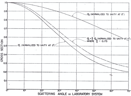
Figure 2. Theoretical differential cross sections corrected for thermal motion of molecules.
For the processing of the image, I used GIMP and LibreOffice both of which are Free and Open Source Software (FOSS). I am a huge fan and advocate of FOSS. Just last week I headed an event in UP on the 25th celebration of Linux Day. I even featured GIMP in the talk that I gave. I told my audience the value of free software and why we should unplug from the sockets of digital imperialism. I think I was able to convince most of them to run Linux and their machines and use the free GIMP rather than the ultimatly expensive Adobe Photoshop.

Figure 3. Linux Day and FOSS Appreciation in UP Diliman.
Going back to the processing of the image, after I loaded it to GIMP, I pointed my mouse to the X and Y tick marks and recorded the values in LibreOffice. In the spreadsheet, I made two separate colums for the real image values (actual tick marks on the image) and the pixel image values both for the X and Y axis. I then produced a plot of those value and displayed the linear equation that would serve as the calibration equations. Figure 4 (a) and (b) show the generated plots and equations.

(a)

(a)
Figure 4. Calibration equations of the X and Y Axis
The next thinkg that I did was to choose a curve to reconstruct since I have three from my image. I chose the middle curve. While still in GIMP, I picked 81 points (back pains and eye strain alert!) from the curve and recorded it in LibreOffice. The calibration equations given above relate the pixel locations to physcial variables. I subtituted the 81 points to the calibration equations and reconstructed the curve shown in Figure 5.

Figure 4. Reconstructed curve from calibrated pixel values of X and Y Axis.
Overall, the activity was easy. The only struggle was finding the image to reconstruct (for my classmates maybe) and listing as many accurate pixel points from the curve. I rate my self 10/10 since I have successfully reconstructed the desired curve from the image. Before I forgot, Ma'am Jing told us that she would give away bonus points to those who are able to overlay the reconstructed image to the original image. Luckily, I am using a very capable free software (LibreOffice) wherein you can change the background of the chart to any desired image. Figure 5 shows the final overlayed image.

Figure 5. Final output with reconstructed image overlayed with the original image.
Since I have done the bonus part, I give my self a score of 12/10. This method of scanning, although may suffice to some applications, is very time and effort consuming. Automating this process is one way to go. This can be done by color subtraction of the curve from the background or even edge detection algorithms. Same idea revolves around the technology of commercial scanners. Instead of pixels, scanners convert reflected intensities to binary digits by using series of mirror, lenses and optical light sources [2].
Acknowledgements:
I would like to extend my sincerest gratitude to the College of Science Library staffs for being so helpful and kind letting me access the materials at their Archive Section.
References:
[1] D. Hurst, et. al., “The Scattering Lengths of the Deuteron,” Canadian Journal of Physics Volume 29 January 1951.
[2] How Stuff Works. "How Scanners Work?". Retrieved from : http://computer.howstuffworks.com/scanner.htm